In this final project we will put in practice most of the concepts learnt so far in the course. It is also a good opportunity to explore how to model vaccination, and to think carefully about resource allocation during public health emergencies. This final exercise is intended to be solved collaboratively, and presented back to the wider group at the end of the day. There are no uniquely correct answer, although there are specific points during the practical where there is a single correct course of action. During the practical copy and paste the code shown into a new script, make the necessary edits or fill the gaps and execute the chunks of code in your own R project.

1. A gastroenteritis outbreak

You lead the outbreak analysis advisory team in your district, where an outbreak of gastroenteritis (GE) has developed over the last month. The index case was reported in a large general hospital in a 66 year old man, who suffered from vomit, diarrhea and dehydration lasting for a period of 2 days. Subsequent cases of similar symptoms have been reported in the same hospital and other hospitals in the district. Outbreak investigation team have recorded the cases occurring at hospitals and stool and blood samples where collected when it was possible.

An initial case control investigation has shown that it is not possible to pin down a single source or common contamination source which has set the alarms for a water-borne gastroenteritis outbreak. A total of 3166 cases have been recorded during the outbreak, of which 79 have produced laboratory samples. The laboratory results show that 91% (71) cases have reported back a positive PCR for Human Norovirus (NoV).

You are handed a small dataset (see below) with the series of cases. Load your data and plot it. download your dataset, and save it in a folder called “data” in your R project.

#load necessary packages
library(ggplot2)
library(reshape2)
library(dplyr)
library(here)
# Install this package to plot and explore contact matrices
install.packages(socialmixr)
library(socialmixr)
 
# Load Epidemic data 
data<-read.csv(here("data","WRITE-HERE-THE-NAME-OF-YOUR-FILE.csv"))
 
# create an X axis for plotting (Barplots need a categorical axis)
data$t<-as.factor(data$Days)
 
# Barplot
ggplot(data, aes(x=t, y=Cases)) + 
  geom_bar(stat = "identity", width=0.2)+
  ylab("reported GE cases") +
  xlab("day")

## 
## Attaching package: 'dplyr'

## The following objects are masked from 'package:stats':
## 
##     filter, lag

## The following objects are masked from 'package:base':
## 
##     intersect, setdiff, setequal, union

## 
## Attaching package: 'socialmixr'

## The following object is masked from 'package:utils':
## 
##     cite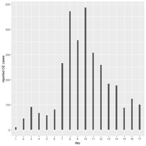

plot of chunk unnamed-chunk-2

2. Calibrate a model for NoV transmission to outbtreak data

As a modeller you are asked to use the existing outbreak data to create and calibrate a model for NoV transmission in different age groups and use it to see if the outbreak can be reproduced by simulation. A systematic review of the existing knowledge on Norovirus has found the following main points: Human Norovirus causes outbreaks of gastroenteritis principally among young children and the elderly. A symptomatic case has a duration of 2 days in average, with an incubation period of no more than 1 day. After a symptomatic period individuals can shed virus in their stools for about 15 days, which makes them slightly infectious but drastically less than a fully symptomatic case.

It is expected for the total size of the outbreak to be much larger, given that only a fraction of the cases of GE get reported or go to hospital. This is even more clear for the elderly who can rapidly deteriorate after contracting GE. For this reason you should correct your out put using previously estimated ratios of community cases per reported case (in the code below).

Below is the code for a SEIAR stochastic, age structured model of Norovirus transmission. The model is programmed using the Odin package, which we have used in previous practicals.

Task 1: By reading the code below, try to interpret what the model structure looks like. Draw an schematic.
Task 2: Fill-in the gaps of data in the code below,, marked with a question (??) symbol. Read carefully the text above to extract the data and convert to meaningful rates.

# Load ODIN package
library(odin)
 
## Create a NoV moodel 
seiar_generator <- odin::odin({
  
  dt <- user(1)
  initial(time) <- 0
  update(time) <- (step + 1) * dt
  
  
  ## Core equations for overall transitions between compartments:
  update(V_tot) <- V_tot + sum(n_SV) + sum(n_RV) - sum(n_VS) - sum(n_VVA) 
  update(S_tot) <- S_tot + sum(n_VS) + sum(n_RS) - sum(n_SE) - sum(n_SV)  
  update(E_tot) <- E_tot + sum(n_SE)  - sum(n_EI) 
  update(I_tot) <- I_tot + sum(n_EI) - sum(n_IA) - sum(n_deathI)
  update(A_tot) <- A_tot + sum(n_IA) - sum(n_AR) - sum(n_deathA)
  update(VA_tot) <- VA_tot +  sum(n_VVA) - sum(n_VAR) - sum(n_deathVA)
  update(R_tot) <- R_tot + sum(n_AR) + sum(n_VAR) - sum(n_RS) - sum(n_RV) 
  
  ## Equations for transitions between compartments by age group
  update(V[]) <- V[i] + n_SV[i] + n_RV[i] - n_VS[i] - n_VVA[i] 
  update(S[]) <- S[i] + n_VS[i] + n_RS[i] - n_SE[i] - n_SV[i]    
  update(E[]) <- E[i] + n_SE[i] - n_EI[i] 
  update(I[]) <- I[i] + n_EI[i] - n_IA[i] - n_deathI[i]
  update(A[]) <- A[i] + n_IA[i] - n_AR[i] - n_deathA[i]
  update(VA[]) <- VA[i] + n_VVA[i] - n_VAR[i] - n_deathVA[i]
  update(R[]) <- R[i] + n_AR[i] + n_VAR[i] - n_RS[i] - n_RV[i]
  
  ## Model outputs for analysis
  update(cum_vaccines[]) <-cum_vaccines[i]+ n_SV[i] + n_RV[i]
  update(new_cases[]) <- n_EI[i] 
  update(cum_cases[]) <- cum_cases[i] + n_EI[i] 
  update(cum_deaths[]) <- cum_deaths[i] + n_deathI[i] + n_deathA[i] + n_deathVA[i]
  
  update(cum_vaccines_all) <- cum_vaccines_all+ sum(n_SV) + sum(n_RV)
  update(new_cases_all) <- sum(n_EI)
  update(cum_cases_all) <- cum_cases_all + sum(n_EI) 
  update(new_reported_all) <- sum(new_reports)
  update(cum_deaths_all) <- cum_deaths_all + sum(n_deathI) + sum(n_deathA) + sum(n_deathVA)
  
  new_reports[]<- n_EI[i] * 1/rep_ratio[i]
  dim(new_reports)<-N_age
  
  
  ## Individual probabilities of transition:
  p_VS[] <- 1 - exp(-delta * dt)  # V to S
  p_SE[] <- 1 - exp(-lambda[i] * dt) # S to E
  p_EI   <- 1 - exp(-epsilon * dt) # E to I
  p_IA   <- 1 - exp(-theta * dt) # I to A
  p_AR   <- 1 - exp(-sigma * dt) # A to R
  p_RS   <- 1 - exp(-tau * dt) # R to S
  p_vacc[] <- 1 - exp(-vac_imm*vac_cov[i] * dt)# vaccination
  p_noromu[]<- 1 - exp(- ((p_IA+p_AR) * cfr[i]/(1-cfr[i])) * dt)# vaccination
  
  ## Force of infection
  m[, ] <- user() # age-structured contact matrix
  s_ij[, ] <- m[i, j] * (I[j] + (A[j] * rho )+ (A[j] * rho * vac_eff) )
  lambda[] <- beta * sum(s_ij[i, ])
  
  ## Draws from binomial distributions for numbers changing between
  ## compartments:
  
  # Flowing out of V 
  n_VS[] <- rbinom(V[i],  p_VS[i])
  n_VVA[] <- rbinom(V[i]-n_VS[i], p_SE[i] * (1-vac_eff))
  
  # Flowing out of S
  n_SE[] <- rbinom(S[i], p_SE[i])
  n_SV[] <- rbinom(S[i]-n_SE[i], if (step > t_vacc) p_vacc[i] else 0)
  
  # Flowing out of E
  n_EI[] <- rbinom(E[i], p_EI)
  
  # Flowing out of I
  n_IA[] <- rbinom(I[i], p_IA)
  n_deathI[]<-rbinom(I[i] - n_IA[i], p_noromu[i])
  
  # Flowing out of A
  n_AR[] <- rbinom(A[i], p_AR)
  n_deathA[]<-rbinom(A[i] - n_AR[i], p_noromu[i])
  
  # Flowing out of VA
  n_VAR[] <- rbinom(VA[i], p_AR)
  n_deathVA[]<-rbinom(VA[i] - n_VAR[i], p_noromu[i]* (1-vac_eff))
  
  # Flowing out of R
  n_RS[] <- rbinom(R[i], p_RS)
  n_RV[] <- rbinom(R[i] - n_RS[i], if (step > t_vacc) p_vacc[i] else 0)
  
  ## Initial states:
  initial(V_tot) <- sum(V_ini)
  initial(S_tot) <- sum(S_ini)
  initial(E_tot) <- sum(E_ini)
  initial(I_tot) <- sum(I_ini)
  initial(A_tot) <- sum(A_ini)
  initial(VA_tot) <- sum(VA_ini)
  initial(R_tot) <- sum(R_ini)
  
  initial(V[]) <- V_ini[i]
  initial(S[]) <- S_ini[i]
  initial(E[]) <- E_ini[i]
  initial(I[]) <- I_ini[i]
  initial(A[]) <- A_ini[i]
  initial(VA[]) <- VA_ini[i]
  initial(R[]) <- R_ini[i]
  initial(cum_vaccines[]) <- 0
  initial(new_cases[]) <- 0
  initial(cum_cases[]) <- 0
  initial(cum_deaths[]) <- 0
  initial(cum_vaccines_all) <- 0
  initial(new_cases_all) <- 0
  initial(cum_cases_all) <- 0
  initial(new_reported_all)<-0
  initial(cum_deaths_all) <- 0
  
  
  ## User defined states - default in parentheses:
  V_ini[] <- user()
  S_ini[] <- user()
  E_ini[] <- user()
  I_ini[] <- user()
  A_ini[] <- user()
  VA_ini[] <- user()
  R_ini[] <- user()
  
  ########## Model parameters (values in brackets are default values) 
  
  beta <- user(0.003)   # transm coefficient
  delta <- user(1/365)  # vaccine immunity dur (~1 yras)
  epsilon <- user( ?? ) #######<------------------------ Fill in incubation
  theta <- user(??)     #######<------------------------ Fill in duration symptoms
  sigma <- user(??)     #######<------------------------ Fill in duration asymp shedding
  tau   <- user(1/365)  # duration immunity
  rho   <- user(0.05)   # rel infect asymptomatic 
  cfr[]  <- user()      # Noro CFR by age 
  vac_eff<-user(0.9)    # Vaccine efficacy for transmission
  vac_cov[]<-user()     # vaccine coverage by age group
  vac_imm  <- user(1/5) # time to vaccine seroconversion (days)
  t_vacc   <- user(2)   # days after case 0 to intro vaccine
  rep_ratio[]  <-user() # cases in community per case reported 
  
  # dimensions of arrays
  N_age <- user()
  dim(V_ini) <- N_age
  dim(S_ini) <- N_age
  dim(E_ini) <- N_age
  dim(I_ini) <- N_age
  dim(A_ini) <- N_age
  dim(VA_ini) <- N_age
  dim(R_ini) <- N_age
  dim(vac_cov)<-N_age
  dim(cfr)  <- N_age  
  dim(rep_ratio)  <- N_age  
  dim(V) <- N_age
  dim(S) <- N_age
  dim(E) <- N_age
  dim(I) <- N_age
  dim(A) <- N_age
  dim(VA) <- N_age
  dim(R) <- N_age
  dim(cum_vaccines) <- N_age
  dim(new_cases) <- N_age
  dim(cum_cases) <- N_age
  dim(cum_deaths) <- N_age
  dim(n_SV) <- N_age
  dim(n_RV) <- N_age
  dim(n_VS) <- N_age
  dim(n_VVA) <- N_age
  dim(n_VAR) <- N_age
  dim(n_SE) <- N_age
  dim(n_EI) <- N_age
  dim(n_IA) <- N_age
  dim(n_AR) <- N_age
  dim(n_RS) <- N_age
  dim(n_deathI)<-N_age
  dim(n_deathA)<-N_age
  dim(n_deathVA)<-N_age
  dim(p_VS) <- N_age
  dim(p_SE) <- N_age
  dim(p_vacc)<-N_age
  dim(p_noromu)<-N_age
  dim(m) <- c(N_age, N_age)
  dim(s_ij) <- c(N_age, N_age)
  dim(lambda) <- N_age
}, verbose = FALSE)

To implement an age-structured model we need a few pieces of information:

1) Age groups: Age structure needs to be defined. It has been decoded that the groups of interest are 0 to 4, 5 to 14, 15 to 64 and over 65s.

2) Age specific rates of contact. If we implement age groups we need to inform the model with the rates at which individuals of certain age group get in effective contact (i.e., the contact sufficient for transmission) with other age groups. This is called a contact matrix. In this practical we are using a widely used source of contact matrices, called POLYMOD. See here. POLYMOD projects contact matrix for over 152 countries. We are using a matrix estimated for Turkiye. It has been adapted to match the age groups of interest. Download the matrix form your materials website and save the csv file in your “data” folder. This contact matrix contains the mean number of contacts that an individual of age i has with another individual of age j in one day. Check the code below and try to interpret the graphic of the matrix.

# Load contact matrix 
cmat<-read.csv(here("data","contact_TUR.csv",sep=""))
 
contact_matrix<-as.matrix(cmat) # Concert to a matrix object
rownames(contact_matrix)<-c("0-4","5-14","14-64","65+") # add age labels
colnames(contact_matrix)<-c("0-4","5-14","14-64","65+") # add age labels
 
# use matrix_plot to plot the contact matrix
matrix_plot(contact_matrix)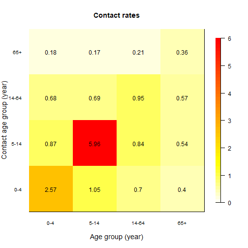

plot of chunk unnamed-chunk-6

Look carefully at the plot above and think what this means for disease transmission.

Now let’s bring together all the other inputs and run the model created in part 1.

In the next part you will try to find the values of beta that best fit the data of the outbreak.

# Seed for random numbers
set.seed(1)
 
# Define total population in the district X of interest
N<-68000
 
n_age<- 4 # number of age groups
 
# Population parameters
            #  0-4  5-14  15-64  65+
pop_distr<- c(0.16, 0.17, 0.63,  0.04) # Population age distribution
pop <- round(N * pop_distr)
 
# Process contact matrix: we need to make sure that the matrix is symmetric 
# i.e., contacts demanded are equal to contacts offered
cmat_sym<-((cmat+t(cmat))/2)
 
# Find per-capita contact rate to input into transmission formula 
# i.e, correcte dto population size in each group
transmission <- as.matrix(cmat_sym )/
  rep(c(t(pop)), each = ncol(cmat_sym))
 
# Noro Case fatality rate (see Lindsay et al https://bmcinfectdis.biomedcentral.com/articles/10.1186/s12879-015-1168-5))
 
# NoV CFR by age group
     #  0-4  5-14  15-64  65+
mu<-c( 0.04, 0.01, 0.03, 0.63)/1000
 
# Reported ratios: cases in the community per case reported in hospital outbreak
# (Assumption: this is not exact but e.g, in the UK it is estimated that for every 
# reported ~280 can be found in the community)
 
          #  0-4  5-14  15-64  65+
rep_ratio<-c(40,  65,   30,    15)

Now that you have all the pieces to run the model

1) Use the code below to explore values of beta that fit best the cases reported in the outbreak (tip: try exploring values between 0.5 and 2)

2) Save your best fitting plot for presentation and your beta value. You will need this later

# Call SEIAR object
seiar0 <- seiar_generator$new(
  V_ini = c(1:n_age)*0,
  S_ini = as.numeric(round(N*pop_distr - c(1,0,0,0))),
  E_ini = c(1:n_age)*0,
  I_ini = c(1,0,0,0),
  A_ini = c(1:n_age)*0,
  VA_ini = c(1:n_age)*0,
  R_ini = c(1:n_age)*0,
  N_age = n_age,
  cfr= mu,
  m=transmission,
  rep_ratio=rep_ratio,
  vac_cov= c(0,0,0,0),
  beta = 0 ## <================ Try different values of beta that fit best in the plot below
)
 
 
# Multiple runs (100)
t_end<- 365 * 2 # sim time (2 years)
 
# Run the model
seiar0_100 <- seiar0$run(0:t_end, replicate = 100)
 
# Variables index
idx<-rownames(seiar0_100[1,,])
 
# PLot reported cases vs data : Iterate through this code until you find the right beta
t_id<-which(idx=="time")
id<- which(idx=="new_reported_all")
mean <- rowMeans(seiar0_100[, id,])
matplot(seiar0_100[, t_id,],seiar0_100[, id,], 
        xlab = "Days", 
        ylab = "Number of GE reported cases",
        type = "l", lty = 1, col="grey",
        xlim=c(0,30),
        ylim=c(0,max(data$Cases)*1.2))
lines(seiar0_100[, 1,1],mean,col="purple")
points(data$Days+5, data$Cases, col = "red", pch = 19)

Now that you have found a good-fitting value for beta , explore some of the transmission dynamics of your calibrated model .

Run the code below to plot total simulated incidence of NoV cases during the outbreak (not corrected by reporting ratios)

# Community incidence
id<- which(idx=="new_cases_all")
mean <- rowMeans(seiar0_100[, id,])
matplot(seiar0_100[, t_id,],seiar0_100[, id,], 
        xlab = "Days", 
        ylab = "Number of cases",
        type = "l", lty = 1, col="grey",
        xlim=c(0,30))
lines(seiar0_100[, 1,1],mean,col="purple")

Modelled cumulative deaths by NoV

# Cumulative NoV deaths
id<- which(idx=="cum_deaths_all")
mean <- rowMeans(seiar0_100[, id,])
matplot(seiar0_100[, t_id,],seiar0_100[, id,], 
        xlab = "Days", 
        ylab = "cumulative of deaths",
        type = "l", lty = 1, col="grey",
        xlim=c(0,365))
lines(seiar0_100[, 1,1],mean,col="purple")

Stacked deaths by age

# Stacked deaths by age 
 
time <- (seiar0_100[, t_id,1])
t<-rep(time,4)
age <-  c(rep(c("0_4") , length(time)), 
          rep(c("5_14") , length(time)),
          rep(c("15_64") , length(time)), 
          rep(c("65+") , length(time)))
deaths <- c( rowMeans(seiar0_100[,which(idx=="cum_deaths[1]") ,]),
             rowMeans(seiar0_100[,which(idx=="cum_deaths[2]") ,]),
             rowMeans(seiar0_100[,which(idx=="cum_deaths[3]") ,]),
             rowMeans(seiar0_100[,which(idx=="cum_deaths[4]") ,]))
df <- data.frame(t,age,deaths)
 
# Stacked cumulative deaths over time by age
ggplot(df, aes(fill=age, y=deaths, x=t)) + 
  geom_bar(position="stack", stat="identity")+
  xlab("days")+ ylab("Cumulative Deaths")
 
 
# Relative stacked cumulative deaths over time by age
ggplot(df, aes(fill=age, y=deaths, x=t)) + 
  geom_bar(position="fill", stat="identity")+
  xlab("days")+ ylab("Proportion of Cumulative Deaths")

Cases of NoV simulated by age group

# cases by age 
time <- (seiar0_100[, t_id,1])
t<-rep(time,4)
age <-  c(rep(c("0_4") , length(time)), 
          rep(c("5_14") , length(time)),
          rep(c("15_64") , length(time)), 
          rep(c("65+") , length(time)))
cases <- c( 1000*(rowMeans(seiar0_100[,which(idx=="cum_cases[1]") ,])/pop[1]),
            1000*( rowMeans(seiar0_100[,which(idx=="cum_cases[2]") ,])/pop[2]),
            1000*(rowMeans(seiar0_100[,which(idx=="cum_cases[3]") ,])/pop[3]),
            1000*(rowMeans(seiar0_100[,which(idx=="cum_cases[4]") ,]))/pop[4])
df <- data.frame(t,age,cases)
 
ggplot(df,aes(color=age, y=cases, x=t)) + 
  geom_line() +
  xlab("days")+ ylab("cumulative incidence rate per 1000 population")

Look carefully at this plots and try to understand

a) what groups are most affected ?

b) What age group drives the outbreak in size?

Before moving to the next step. Run the code below to create useful model output that you will use as your baseline estimations in the next part.

# Analysis output
 
id<- which(idx=="cum_deaths_all")
base_deaths <- mean(seiar0_100[365 ,id, ]) # cumulative deaths by NoV after one years 
 
id<- which(idx=="cum_cases_all")
base_cases <- mean(seiar0_100[365 ,id, ]) # cumulative cases by NoV after one years 
 
id<- which(idx=="cum_vaccines_all")
base_doses <- mean(seiar0_100[365 ,id, ]) # cumulative vaccine doses (0) after one years

3. A new vaccine becomes available

In this part of the project you are asked to assess potential vaccination scenarios and make a decision on the most efficient way to use your resources.

The vaccine development pipeline for Norovirus currently has at least three potential formulations in phase III trials. This formulations include inactivated virus, mRNA and VLP (virus like particles) types of vaccines. They all include the genogroup GII.4 and either GI.3 or GI.1 genogroup. GII.4 is the cause of most epidemics around the world. For simplicity we are not modelling genogroups or variants in this exercise.

You are informed that two vaccine formulations have become available :

NoVax Vaccine: In preliminary immunogenecity studies it has shown good antibody (AB) response, which peaks at around 5 days after the first dose. Phase III trials have shown an underwhelming efficacy of 75%
Vomax Vaccine: This vaccine has a shown a very high efficacy of 92%, however the immunological response is much slower given the method of production and it takes ~12 days to reach protective AB values

It is expected that new outbreaks of contaminated waters will occur again in your district and you are asked to use your model to retrospectively assess how a potential vaccine could prevent cases and save lives in a similar outbreak.

For this you need to propose three scenarios of vaccination where you explore different age specific vaccine coverage with either NoVax or Vomax vaccine. For each scenario you will estimate:

Total cases prevented over one year (relative to baseline)
Total deaths averted over one year (relative to baseline)
Total doses delivered
Doses per case and death averted

Importantly, you are informed that only 100,000 doses of either vaccine will be made available, so any decision you make needs to consider this.

Below you will see the code necessary to create each of the three scenarios and estimate the impact indicators.

iterate through this scenarios as necessary until you find your answer.

Tip: think carefully about the dynamics of transmission and what groups are most affected by incidence and mortality

At the end your group will prepare a 5 min (max) presentation in which you will present:

a) best model fit to data

b) Table with Three scenarios of analysis and its impact

c) Choose only one scenario and give your rationale in epidemiological terms

Scenario 1

## Scenario 1
 
seiar1 <- seiar_generator$new(
  V_ini = c(1:n_age)*0,
  S_ini = as.numeric(round(N*pop_distr - c(1,0,0,0))),
  E_ini = c(1:n_age)*0,
  I_ini = c(1,0,0,0),
  A_ini = c(1:n_age)*0,
  VA_ini = c(1:n_age)*0,
  R_ini = c(1:n_age)*0,
  N_age = n_age,
  cfr= mu,
  m=transmission,
  rep_ratio=rep_ratio,
  vac_cov= c(0,0,0,0),## <------- Chose coverage of vaccination in different age groups (0 to 1)
  vac_eff = 0,       ## <------- Fill vaccine efficacy (NoVax or Vomax)
  vac_imm = 0,       ## <------- Fill rate to AB protection (NoVax or Vomax) (1/days)
  beta = 0           ## <--------Fill with your best fitted beta from part 2
)
 
# Run the model
seiar1_100 <- seiar1$run(0:t_end, replicate = 100)
 
# Analysis output
id<- which(idx=="cum_deaths_all")
sc1_deaths <- mean(seiar1_100[365 ,id, ]) ## Cumulative deaths after 1 year
 
id<- which(idx=="cum_cases_all")
sc1_cases <- mean(seiar1_100[365 ,id, ]) ## Cumulative cases after 1 year
 
id<- which(idx=="cum_vaccines_all")
sc1_doses <- mean(seiar1_100[365 ,id, ]) ## Cumulative doses after 1 year
 
sc1_avdeaths<-base_deaths-sc1_deaths ## Deaths averted after 1 year
 
sc1_avcases<-base_cases-sc1_cases    ## Cases averted after 1 year
 
dose_per_avdeath1<- sc1_doses/sc1_avdeaths ## doses needed to avert 1 death 
 
dose_per_avcase1<- sc1_doses/sc1_avcases ## doses needed to avert 1 case

Scenario 2

## Scenario 2
 
seiar2 <- seiar_generator$new(
  V_ini = c(1:n_age)*0,
  S_ini = as.numeric(round(N*pop_distr - c(1,0,0,0))),
  E_ini = c(1:n_age)*0,
  I_ini = c(1,0,0,0),
  A_ini = c(1:n_age)*0,
  VA_ini = c(1:n_age)*0,
  R_ini = c(1:n_age)*0,
  N_age = n_age,
  cfr= mu,
  m=transmission,
  rep_ratio=rep_ratio,
  vac_cov= c(0,0,0,0),## <------- Chose coverage of vaccination in different age groups (0 to 1)
  vac_eff = 0,       ## <------- Fill vaccine efficacy (NoVax or Vomax)
  vac_imm = 0,       ## <------- Fill rate to AB protection (NoVax or Vomax) (1/days)
  beta = 0           ## <--------Fill with your best fitted beta from part 2
)
 
# Run the model
seiar2_100 <- seiar2$run(0:t_end, replicate = 100)
 
# Analysis output
id<- which(idx=="cum_deaths_all")
sc2_deaths <- mean(seiar2_100[365 ,id, ]) ## Cumulative deaths after 1 year
 
id<- which(idx=="cum_cases_all")
sc2_cases <- mean(seiar2_100[365 ,id, ]) ## Cumulative cases after 1 year
 
id<- which(idx=="cum_vaccines_all")
sc2_doses <- mean(seiar2_100[365 ,id, ]) ## Cumulative doses after 1 year
 
sc2_avdeaths<-base_deaths-sc2_deaths ## Deaths averted after 1 year
 
sc2_avcases<-base_cases-sc2_cases    ## Cases averted after 1 year
 
dose_per_avdeath2<- sc2_doses/sc2_avdeaths ## doses needed to avert 1 death 
 
dose_per_avcase2<- sc2_doses/sc2_avcases ## doses needed to avert 1 case

Scenario 3

## Scenario 3
 
seiar3 <- seiar_generator$new(
  V_ini = c(1:n_age)*0,
  S_ini = as.numeric(round(N*pop_distr - c(1,0,0,0))),
  E_ini = c(1:n_age)*0,
  I_ini = c(1,0,0,0),
  A_ini = c(1:n_age)*0,
  VA_ini = c(1:n_age)*0,
  R_ini = c(1:n_age)*0,
  N_age = n_age,
  cfr= mu,
  m=transmission,
  rep_ratio=rep_ratio,
  vac_cov= c(0,0,0,0),## <------- Chose coverage of vaccination in different age groups (0 to 1)
  vac_eff = 0,       ## <------- Fill vaccine efficacy (NoVax or Vomax)
  vac_imm = 0,       ## <------- Fill rate to AB protection (NoVax or Vomax) (1/days)
  beta = 0           ## <--------Fill with your best fitted beta from part 2
)
 
# Run the model
seiar3_100 <- seiar3$run(0:t_end, replicate = 100)
 
# Analysis output
id<- which(idx=="cum_deaths_all")
sc3_deaths <- mean(seiar3_100[365 ,id, ]) ## Cumulative deaths after 1 year
 
id<- which(idx=="cum_cases_all")
sc3_cases <- mean(seiar3_100[365 ,id, ]) ## Cumulative cases after 1 year
 
id<- which(idx=="cum_vaccines_all")
sc3_doses <- mean(seiar3_100[365 ,id, ]) ## Cumulative doses after 1 year
 
sc3_avdeaths<-base_deaths-sc3_deaths ## Deaths averted after 1 year
 
sc3_avcases<-base_cases-sc3_cases    ## Cases averted after 1 year
 
dose_per_avdeath3<- sc3_doses/sc3_avdeaths ## doses needed to avert 1 death 
 
dose_per_avcase3<- sc3_doses/sc3_avcases ## doses needed to avert 1 case